

A landmark realization in science often occurs when a passive, descriptive measurement of a system is discovered to be the key to its active, underlying mechanism. This article details such a realization at the heart of Fractional Scaling Digital Signal Processing (FSDSP). We explore the journey of the scaling exponent \beta from a well-known empirical statistic—used to characterize the power-law behavior of signals on a log-log plot—to its identification as the active, operational exponent on the Laplace operator s. This pivotal insight bridges the gap between empirical observation and operational calculus. It transforms our understanding of natural systems, shifting from an incomplete “\frac{1}{f}-noise” model to a more complete “\frac{1}{s}-noise” framework that unifies magnitude and phase. We demonstrate how this realization allows \beta to function as a direct fractional operator, enabling FSDSP to perform any order of fractional integration or differentiation on a signal. This principle is the foundational innovation underpinning sNoise Research Laboratory’s (sNRL) patents and its capacity to create true “white box” models of physical reality.
1.0 A Conceptual Framework for Fractional Calculus
1.1 The Origins of a 300-Year-Old Idea
The conceptual seeds of fractional calculus, the generalization of differentiation and integration to non-integer (and even complex) orders, were sown remarkably early in the history of calculus itself. The very notion is often traced back to a seminal exchange in 1695 between Gottfried Wilhelm Leibniz, one of the principal architects of classical calculus, and the Marquis de L’Hôpital. L’Hôpital, intrigued by Leibniz’s \frac{d^ny}{dx^n} notation for integer-order derivatives, posed the question: “Can the meaning of derivatives with integer order be generalized… What if the order will be \frac{1}{2}?”. Leibniz, in a letter dated September 30, 1695—a date often celebrated by historians as the symbolic birthday of fractional calculus—famously replied: “It will lead to a paradox, from which one day useful consequences will be drawn”.
This prophetic insight, acknowledging both the apparent conceptual difficulties and the latent potential of fractional orders, set the stage for centuries of mathematical exploration. Early contributions and further inquiries came from luminaries such as Euler, Laplace, Fourier, Lacroix, Abel, Liouville, and Riemann, who grappled with defining these non-integer operations, often in the context of specific mathematical problems or functions. These early explorations typically focused on developing definitions within the time domain, such as the Riemann-Liouville and Caputo fractional derivatives, or discrete approximations like the Grünwald-Letnikov definition. While foundational, these time-domain approaches often present complexities in application, particularly for systems with intricate memory effects or those more naturally analyzed via their frequency characteristics. The “useful consequences” Leibniz envisioned remained largely theoretical and elusive until the evolution of more tractable frequency-domain methods and the advent of the modern computer.
1.2 The Language of Nature: Memory and Scaling Behavior
The evolution of fractional calculus eventually led to powerful formulations in the frequency domain, particularly through the Laplace and Fourier transforms. This shift allowed for a more direct and often more tractable analysis of how systems exhibiting fractional-order dynamics respond to inputs, paving the way for modern applications. While the established frameworks of modern physics have provided profound insights, their traditional reliance on integer-order calculus is insufficient to fully capture the intricate dynamics and inherent complexities observed in natural and stochastic systems. Nature, in its diverse manifestations, often exhibits behaviors characterized by long-range correlations, memory effects, and non-local interactions—phenomena that extend beyond the descriptive capabilities of conventional calculus. This suggests that the “language” in which the universe is written is more nuanced, requiring mathematical tools that can accommodate non-integer orders of operation.
Fractional Calculus (FC) is that language. As a superset of and an extension to traditional calculus, fractional calculus allows for fractional differentiation and integration at arbitrary non-integer (fractional) orders. This superset is not merely a mathematical curiosity but offers unique solutions unavailable to integer-order calculus alone and is essential for accurately modeling memory effects, complex dynamic phenomena, and natural scaling behavior prevalent in the physical world. Scaling behavior is a property where a system’s dynamics exhibit a consistent form of complexity regardless of the scale at which they are observed, often following a mathematical power-law relationship.
To quantify this, we use a single, powerful parameter called the scaling exponent (\beta). This scaling exponent is a precise measurement that describes not only how much a system’s behavior changes with scale, effectively capturing the extent of its underlying memory and dynamic nature in a single number, but also why or the actual mechanisms or processes that generate such behavior. Nature, it is posited, inherently performs these fractional-order operations, continuously processing information and energy via these fractional calculus principles operating in the complex frequency, and the key to understanding them lies in this scaling exponent.
As will be elaborated in the next section, the most effective way to measure and operationalize this scaling exponent is by analyzing a system’s output in the frequency domain. This analysis reveals a fundamental limitation in the traditional “\frac{1}{f}-noise” model and points toward a more complete framework operating in the complex frequency, or Laplace, domain (s) that includes the scaling exponent \beta. Consequently, the power of \beta serves not only as a universal descriptor of scaling processes but as a fundamental universe descriptor, hinting at a remarkably simple yet profound underlying computational mechanism for complex natural and cosmic phenomena.
2.0 The Scaling Exponent β: A New Perspective
2.1 The Incompleteness of \frac{1}{f} Noise
The outputs of many natural systems, when analyzed in the frequency domain, exhibit scaling behaviors what is commonly termed “\frac{1}{f}-noise” or “pink noise,” where power spectral density is inversely proportional to frequency P(f) ∝ \frac{1}{f}. While this \frac{1}{f} nomenclature is widespread, it is an oversimplification of the underlying processes. Historically, signal analysis focused on simple, real frequencies, f, and the magnitude or power of the spectrum. However, this approach neglects crucial phase information and the more complete representation afforded by complex frequencies. In other words, by portraying scaling behaviors as only \frac{1}{f}-noise, we are using only one quarter to half of the information actually present in the signal, depending on how we calculate \frac{1}{f} scaling behavior.
2.2 The Shift to \frac{1}{s} Noise and the Complex Frequency Domain
This oversimplification of the mathematical models requires a fundamental shift in perspective: natural systems exhibiting such scaling behaviors are more accurately and comprehensively described not by “\frac{1}{f}-noise”, but by “\frac{1}{s}-noise,” where s is the Laplace operator (s = \sigma + j\omega) representing complex frequency. The real part, \sigma, accounts for damping or growth, while the imaginary part, j\omega (where \omega is the angular frequency and j is the imaginary unit), accounts for oscillation. While for many frequency response analyses in FSDSP, \sigma is often set to zero to focus on the steady-state oscillatory behavior (s = j\omega), the full complex variable s can account for systems with inherent exponential growth or decay, a potential avenue for describing even more intricate system dynamics. This transition from f to s is fundamental because nature appears to operate not just on magnitudes at real frequencies but on the complex interplay of magnitudes and phases within the complex frequency domain.
The operations within this \frac{1}{s}-noise framework are governed by Fractional Scaling Digital Signal Processing (FSDSP), a patented framework of equation-based algorithms developed by Dr. Jeffrey Smigelski. FSDSP operates fundamentally within this complex frequency (Laplace) domain, leveraging the unique properties of fractional operators via the scaling exponent \beta to describe and enact the processes believed to govern natural systems and the universe itself. FSDSP employs fractional calculus to allow for exact fractional filtering—including fractional scaling, fractional phase shifting, fractional integration, or fractional differentiation—to be performed on any signal by precisely adjusting magnitude and/or phase for each individual frequency to any decimal level. The “useful consequences” of fractional calculus that Leibniz envisioned are now beginning to be fully realized through such computational frameworks.
2.3 The Scaling Exponent \beta as an Empirical Measurement
The concept of scaling behavior originates in fractal geometry and describes systems whose properties are consistent across different scales of observation. This consistency is described by a scaling factor—a number that tells you how much you need to “zoom in” or “zoom out” to see repeating patterns. The most basic form of this is self-similarity, where the same scaling factor is applied to all dimensions where an object or process appears identical at different levels of magnification. A more nuanced form, common in natural data like time series, is self-affinity, where different scaling factors are required for different dimensions (e.g., the horizontal time x-axis versus the vertical amplitude y-axis). A classic example from geophysics is quantifying the “roughness” of a mountain range. A young, rugged range like the Rocky Mountains has a different, “rougher” scaling behavior than an older, “smoother”, and more weathered range like the Appalachians. This roughness is a quantifiable, empirical measurement. In signal processing, this same principle is used to quantify the “roughness” of a signal or time series. A “rough” signal is dominated by high frequencies (\beta1). A signal with equal power at all frequencies (\beta=0) can be considered perfectly random, a white noise, without a characteristic texture.
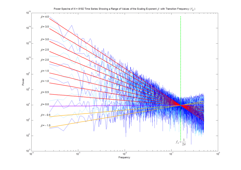
Many natural and stochastic signals or time series exhibit this property as power-law scaling, a form of self-affinity where the signal’s characteristics are consistent across different scales. A standard method for characterizing these signals is to perform a linear least-squares fit of their log-log power spectrum of power (y) vs frequency (x). This technique yields a single empirical descriptor: a slope. Whether analyzing a natural system or a digital signal, the scaling exponent \beta is defined as the negative of this slope when plotted on a log-log scale. A power law is the only function that plots as a straight line on a log-log plot, making this a robust method for quantifying scaling behavior. It is critical to note the relationship between power and magnitude: since power is proportional to magnitude squared, the slope of the power spectrum (\beta) is exactly double the slope of the magnitude spectrum. Historically, \beta has been used as a passive measurement to classify a signal’s “noise type”—such as pink noise (\beta=1) or Brownian motion (\beta=2) or white noise (\beta=0)—and to quantify the degree of “memory” or long-range dependence within the system.
It is crucial to understand that the scaling exponent is not limited to integer-only values but can be any fractional (decimal) number. A fractional \beta suggests that the system’s behavior or processed that produced the measured output lies somewhere in between the well-defined integer states, representing the first glimpse into the power of fractional scaling. This net \beta can be seen as the result of multiple combined processes within the system across different frequency scales leading to an overall fractional calculus-based behavior of the system. Such systems may exhibit self-organized criticality, leading certain \beta values (e.g., \beta=1 for pink noise) to emerge naturally as stable states of the computational dynamics that make up the data being measured.
It is also important to understand that the observed \beta values in natural systems are often emergent properties. While pure, integer-order operations drive a system towards distinct states—pure differentiation towards \beta=-2 and pure integration towards \beta=+2, the fractional values observed in complex reality arise from the dynamic interplay, superposition, and feedback loops of these fundamental operations. A system’s final, measured scaling fractional behavior is therefore the net result of multiple, interacting processes.
3.0 The Landmark Realization: Unifying Measurement and Mechanism
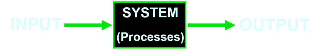
3.1 System Dynamics: Isolating the System’s Transfer Function
A system’s behavior can be described by its transfer function, H(s), which is the ratio of its output, O(s), to its input, I(s): H(s) = \frac{O(s)}{I(s)}
In terms of scaling exponents, this relationship is additive: \beta_{output} = \beta_{input} + \beta_{system}.
3.2 The Measured \beta as the Operational Exponent in Fractional Scaling Digital Signal Processing
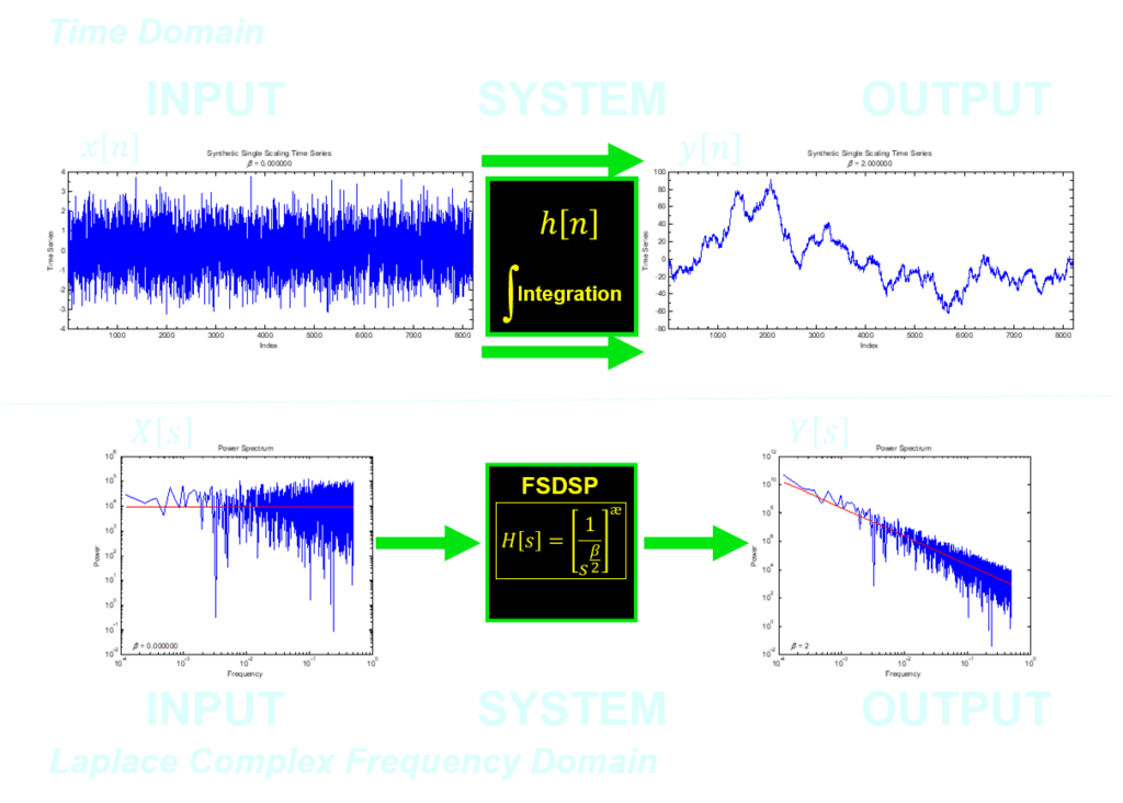
At the heart of FSDSP is the Laplace transfer function for an integrator: \frac{1}{s} which is standard in control theory. It turns out, that after some derivations and mathematical proofs, one can show that the scaling exponent \beta, the same one that is measured from a linear least-squares fit in log-log space, is actually the exponent of the Laplace operator s. This pivotal insight transformed \beta from a passive descriptor of noise into an active, operational component of a transfer function. It turned a diagnostic tool into a generative and manipulative one. This is the “useful consequence” that Leibniz prophesied over three centuries ago.
The core intellectual breakthrough of FSDSP was the realization that the empirically measured scaling exponent \beta from the linear least-squares fit of the power spectrum is not merely a descriptive statistic. Rather, \beta is precisely the exponent that governs the Laplace operator s within the system’s complex frequency domain transfer function.
In fact, the Laplace equation for a fractional integrator (and fractional differentiator) is: \frac{1}{s^{\frac{\beta}{2}}}where the scaling exponent \beta becomes a pivotal parameter. This single parameter, \beta, precisely quantifies “how much” of a fractional integration (if \beta> 0) or fractional differentiation (if \beta< 0) a system performs on an input. This focus on the order of the operation (the value of \beta> 0) rather than just the operands (e.g., + or -) provides deeper insight into system dynamics. The foundational FSDSP transfer function: H(s) = \frac{1}{s^{\frac{\beta}{2}}} can therefore also be written as: H(s) = \frac{1}{s^{\alpha}} where \alpha = \frac{\beta}{2}. In this form, the scaling exponent \alpha is expressed directly as the negative of the slope of the magnitude spectrum.
3.3 The Power of \beta as a Fractional Operator
This realization—that a measured slope can be used to do fractional calculus on a signal—is the operational heart of FSDSP. The scaling exponent \beta is not just a descriptor; it is a fractional operator. By setting the value of \beta in the foundational FSDSP transfer function, H(s) = \frac{1}{s^{\frac{\beta}{2}}}, we can define and execute any degree of fractional integration or differentiation on any input signal. This is important as one realizes that the process of integration or differentiation is simply due to the sign, being + or -, of the exponent \beta on the Laplace operator s. By just changing the sign of the scaling exponent \beta, one can switch from integration to differentiation.
Thus, the entire complexity of a fractional-order system governed by fractional calculus is captured in this elegant, tunable, scaling exponent \beta.
| Set \beta to: | The FSDSP transfer function H(s) = \frac{1}{s^{\frac{\beta}{2}}} performs: | This corresponds to: |
|---|---|---|
| \beta = -2 | Pure, single differentiation | Blue Noise |
| -2<\beta<0 | Fractional differentiation | |
| \beta = 0 | Passes the input signal to the output signal unchanged | White Noise |
| 0 < \beta < 2 | Fractional integration | |
| \beta = 1 | Half-integration | Pink Noise |
| \beta = 2 | Pure, single integration | Brownian Motion |
| 2 < \beta < 4 | “Double” fractional integration | |
| \beta = 3 | One-and-a-half integrations | Black Noise |
| \beta = 4 | Pure, double integration | |
| \beta > 4 | Beyond double integration | Order of Operations = \frac{\beta}{2} |
3.4 The Relationship of Magnitude and Phase of the Fractional Operator to \beta
When the foundational FSDSP transfer function, H(s) = \frac{1}{s^{\frac{\beta}{2}}}, is solved for its constituent parts, we can define the exact magnitude and phase at any frequency.
Given that s is a complex frequency, we can solve the transfer function for magnitude (M_{(\omega)}) and phase (\theta_{(\omega)}) using Euler’s identity.
When solved for Magnitude M_{(\pm\omega)}: M_{(\pm\omega)} = \frac{1}{\omega^{\frac{\beta}{2}}} where \omega is angular frequency, the \pm indicated these frequencies are both positive and negative.
When solved for Phase \theta_{(\pm\omega)}: \theta_{(+\omega)} = -\beta \frac{\pi}{4} for positive angular frequencies (+\omega) and: \theta_{(-\omega)} = \beta \frac{\pi}{4} for negative angular frequencies (-\omega).
In terms of denoting the sign on the complex angular frequency (\omega), this is due to what is called even symmetry in the real or x-component of the complex number and odd symmetry in the imaginary or y-component of the complex number spanning the positive and negative frequencies directly from Euler’s identity.
The fact that the scaling exponent \beta, derived from the power spectrum, directly solves for the precise phase shift \theta at each angular frequency \omega is not inconsequential, but a foundational mathematical property of power-law systems when modeled in the complex frequency domain. This inherent link, a direct consequence of the even and odd symmetries described by Euler’s identity, proves that a system’s magnitude and phase responses are not independent variables but are two facets of the same underlying dynamic, governed by a single scaling parameter. It is this self-consistent relationship that allows FSDSP to both model and control real-world systems with such high fidelity.
4.0 Conclusion: A New Foundation for Signal Processing and AI
The landmark realization that a passive, statistical measurement (\beta) from the linear-least squares fit is the active, operational exponent in the calculus of a system is the core innovation that underpins all of sNRL’s patents. It bridges the gap between empirical observation and operational calculus (and operational fractional calculus), allowing us to move from characterizing systems to generating and controlling them with mathematical precision. This insight provides a new, more fundamental way to model the world.
By extension, this provides a more powerful and physically grounded toolkit for the future of Artificial Intelligence. In an era dominated by opaque “black box” models, this verifiable, equation-based framework offers a path toward a “white box” paradigm where AI’s reasoning is no longer a matter of faith, but of provable mathematics. By giving AI a language that inherently understands the memory, complexity, and scaling behaviors of the real world, we are not just improving its accuracy; we are enhancing its fundamental ability to learn, predict, and interact. In the same way that the discovery of fractals gave us the language to describe the geometry of nature, FSDSP provides the language to describe nature’s dynamics through time.
Dr. Jeffrey Smigelski is the founder of the sNoise Research Laboratory (sNRL) and the sole inventor of the patented Fractional Scaling Digital Signal Processing (FSDSP) framework. FSDSP is a powerful computational implementation of Fractional Calculus, which his work identified as the fundamental mathematics of natural systems. His pioneering research established the connection between empirically measured scaling exponents and operational fractional calculus, creating a new paradigm to precisely model, filter, synthesize, and interact with the physics of real-world systems through an equation-based framework, leading to advancements in signal processing, fractional order control systems, and AI.